Written by Steinar Thorvaldsen,
2004. Last updated: Jan. 2006.
Dept. of
Mathematics and Statistics
University of Tromsø - Norway.
MendelHMM is a Hidden Markov Model (HMM) tutorial toolbox for Matlab. These pages describe the graphical user interface (GUI) and the main operations of the program. The toolbox is free for academic use. Ref.: S. Thorvaldsen: A tutorial on Markov models based on Mendel's classical experiments. Journal of Bioinformatics and Computational Biology, Vol. 3, No. 6 (2005), 1441-1460.
To run the program you should make the following steps:
1.
Download the program to your local PC and install (unzip) it in a directory like …\mendel
2. Run Matlab v. 6.5 or later
3. Set working directory to ...\mendel (root directory of the toolbox)
4. Type "mendelHMM"
When you type "mendelHMM" in Matlab command window the
main window of GUI will appear. In left part of main window there is a
frame containing controls for loading and managing training data. On right there
is a frame containing controls for managing the Hidden Markov model. Button "
>Estimate (EM)>" runs estimation of model from the selected training set.
Baum Welch algorithm is used starting from the pre-selected number of states and
initialization method, but any other values of hidden parameters are ignored.
Button "<Sample (new)<" serves for producing new training sets according to selected
HMM model and sample size.
Main window of the program. There are buttons for loading models and training sets, viewing individual sequences and results.
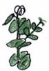
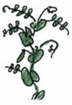
In his historic experiment, Gregor Mendel (1822-1884) examined 7 simple traits in the common garden pea (Pisum). A trait (called phenotype) is one which occurs either in one variation or another, with no in-between. These plants are naturally self-pollinating and exhibited traits which occur in very distinct forms:
|
Experiment number |
Sample size N in F2-generation |
Dominant expression |
Recessive expression |
|
1 Form of ripe seed |
7324 |
smooth |
wrinkled |
|
2 Colour of seed albumen |
8023 |
yellow |
green |
|
3 Colour of seed coat |
929 |
grey |
white |
|
4 Form of ripe pods |
1181 |
inflated |
constricted |
|
5 Colour of unripe pods |
580 |
green |
yellow |
|
6 Position of flowers |
858 |
axial |
terminal |
|
7 Length of stem |
1064 |
tall |
dwarf |
Today we know that the recessive expressions most often are mutations in the DNA molecule of the gene, as it is well known for Mendel’s growth gene (trait 7) where a single nucleotide G is substituted with an A. The consequence is that the 3D structure of the enzyme is changed, and no biochemical reaction can take place.
In his experiment Mendel also studied in more detail the plant seeds with two and three heredity factors simultaneously. When he studied two traits he used 1 and 2, and three traits 1, 2 and 3 in the table above.
The estimate of a statistical model according to a training set
Strictly speaking, the actual model and the actual sequence of hidden state values cannot be found from knowledge of the sequence of observations. The optimal model can only be looked for in a certain probabilistic sense. To search for the most probable model is one of the natural and much used tasks in Markov modeling. In an ideal case the model is derived from knowledge about the objects we study and its configuration. But the available knowledge is insufficient in many practical situations. However, the knowledge can be improved in relation to our training data. This process is called learning.
There are two main types of learning. The first one, the supervised learning, operates with a training set consisting of pairs (xi, yi), where yi is a sequence of observations and xi is a sequence of corresponding states. The second possibility, the unsupervised learning, works with sequences of observations, yi, only. In our example this case is adopted. An important question is the source of the training data, and how it may influence the choice of the proper learning algorithm. The maximum likelihood (ML) estimate is suitable if the training data are random samples from a probability distribution that can be searched for.
Supervised ML estimation is a pure counting of relative frequency of occurrence of events. Unsupervised learning is provided by ML estimation and the Baum-Welch re-estimation algorithm, and it is a special case of the EM algorithm (Expectation Maximization). The algorithm can be viewed as an iterative adaptation of the model to fit the training data. A HMM may often be slow to estimate because of its large number of parameters and many local maxima.
A view of the model parameters estimated by MendelHMM is available from the program:
EM-estimation of model parameters based on two phenotypes and 50 sequences each of length 7. The results are very sensitive to the initial values.
We can achieve a higher efficiency in the optimization methods by using the special properties of the functions that arise in biology. But global optimization is in its infancy, and rapid progress is expected on this field by introducing techniques like data perturbation for escaping local maxima (Simulated Annealing). Simulated Annealing (Kirkpatrick et al., 1983) is an established paradigm for introducing randomness into optimization, by performing a random tour of the search space. But it has been proved that finding the globally-optimal ML parameters is NP-hard (Day 1983), so initial conditions matters a lot for success. Simulated Annealing is not implemented in the toolbox mendelHMM. But initial values may be chosen by two methods, either by random or by a dominant diagonal method.
The sampling of new training data
The toolbox may also produce new data samples from our Markov model by running through it in a probabilistic way. A graphical view of the data sequences can also be provided.
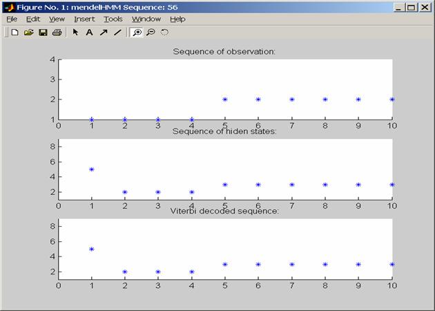
A sequence sample distribution of observations and hidden states from the mendelHMM model with two genes (4 phenotypes and 9 genotypes).
There are some fundamental problems that
has to be solved in the HMM process. The first is the problem of sequence
evaluation, and the Mendel experiment can as an
illustration give us
a simple example of such evaluation, often called the forward/backward
procedure. If we in the case of one gene have a sequence of dominant (A) and
recessive (a) observations:
y = (A, A, a, a, a)
Note that when writing a single letter A in bold,
we mean the phenotype and not the genotype. How do we calculate the probability that the sequence is
derived from the model? In this particular Mendel model we have initial state vector
p,
probability state transition matrix PS, and emission probabilities PE:
The first column in PE tells that all genotypes of type number
1 (AA) and type 2 (Aa) will be observed as phenotype 1(A), and and the
second column tells that all genotypes of type 3 (aa) will be observed as
phenotype 2 (a).
In this simple case only one possible
state path can hide behind the given observations:
(0 1 0) → (0 1 0) → (0 0 1) → (0 0 1) → (0 0 1), and summing up the probabilities gives:
As mentioned earlier, the actual sequence of hidden values cannot be found from knowledge of the sequence of observations and the corresponding Markov model. The optimal sequence can only be looked for in a certain probabilistic sense. The search for the most probable sequence is another of the natural questions in HMM. The Viterbi algorithm solves this task. The algorithm uses dynamic programming and can be interpreted as search for the shortest path.
In our Mendel example, we might be given
a sequence of dominant observations:
y = (A, A, A, A, A)
How do we find the most probable sequence of states (e.g. genotypes)? A predicted path through the HMM should estimate what the genotype sequence are in the emitted symbol sequence. We decode the observed symbol sequence to obtain the states, and choose the path with the highest probability.
Analyzing an observation sequence by the Viterbi algorithm. The solution of the bet state path is shown with bold face.
We are using the best previous path (up to position t) to find the best possible score and path at position t+1. The sequence start by default in state p, and we construct a table of the possible paths, each with a pointer from the previous position that generated it. After constructing the table, the optimal state sequence will be found by backtracking.
A sequence sample of observations and hidden states from the mendelHMM model with 4 phenotypes and 9 states. The Viterbi prediction based on phenotypes alone is also shown, and is very accurate in this example.
More on the Mendel experiment
Gregor
Mendel was an Augustinian monk. His monastery was a centre of
learning and scientific endeavor, and many of its members were teachers at the
local High School or at the Philosophical Institute. He studied science at the
University of Vienna, where he among other attended lectures on experimental
physics by Doppler.
When working on the questions of inheritance, Mendel used combinatorics as his main mathematical tool. Recognizing the value of quantitative analysis, Mendel created a mathematical model for the transmission of heritable traits, based on the concepts of probability. Access to a re-sampled version of Mendel’s data sets is available in our program. Mendel’s original "raw" data are lost, and we first have to regenerate them with the same sample size and ratios as reported in his paper. The genotypes are the (hidden) state sequences, and the phenotypes are the observed symbols. The transition and emission probabilities may be estimated from the sequences of observations, and the number of hidden states may be varied.
In his science Mendel is considered to be a careful collector of data, a thinker in quantitative terms, and an analyzer of observational data by statistical treatment. By the statistical analysis of large numbers, he succeeded in extracting laws from apparently random phenomena. This method is quite common today, but at Mendel's time it was entirely novel. Most biologists of his time were busy describing and categorizing their qualitative observations, statistical ideas combined with quantitative measurements were foreign ground. Mendel was the first to apply statistical analysis to the solution of a basic biological problem and to explain the significance of such a numerical ratio (Gillispie 1974, vol. IX p. 281). He deduced that the sex cells somehow changed from having a double dose of heredity factors to having only one. Mendel could not tell exactly how this occurred - nobody could tell until 25 years later when the process of reduction division in sex cells was described. But Mendel knew that such a change was necessary if the mathematics was to work. The modern words "gene", "genotype" and "phenotype" were introduced as late as 1909 by Wilhelm Johannsen, professor of plant physiology at Copenhagen Agricultural College.
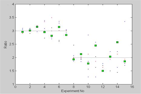
Data plots from the first two parts Mendel's experiment (squares) together with five separate numerical experiments (dots) based on the Markov model with the same sample size as in Mendel's experiment. Experiment 1-7 gives the dominant/recessive ratio. In experiment 8-15 only the dominants are tested future, and thereby determining the ratio between the pure dominant/hybrid dominant. Experiment 12 was repeated and is shown as number 15. The sample size in experiment 1-7 is great (between 8023 and 580), and is less in experiment 8-15 (between 565 and 100).
In his paper Mendel also studied in detail data from two and three independent pair of genes. In the case of two
genes, the plants on the genotype level can be in one of nine states: S={AABB,
aABB, aaBB, AAbB, aAbB, aabB, AAbb, aAbb, aabb}. By standard combinatorics,
the transition matrix can be written:

Here four of the states are absorbing.
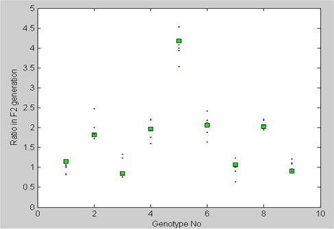
Genotype frequency counts in the F2 generation with two independent genes (9 genotypes). The counts are shown in fractions of 16. Mendel's experiment (squares) had a sample size of 529 plants. Five separate numerical simulations based on the Markov model with the same sample size as in Mendel's experiment are also shown (dots).
The problem created by the fact that Mendel changed his sample size between the subsequent generations, is overcome in the toolbox by restricting our Markov chains to the minimum sampling number within first three generations. And in each experiment and generation the frequencies are preserved as reported by Mendel in his paper. In this way the sample size is like this:
1 gene 2 genes 3 genes Trait 1 2 3 4 5 6 7 1 and 2 1, 2 and 3 Sample size 756 691 132 134 136 132 135 529 639
After 1871 Mendel also conducted experiments with bees, hoping to verify his theory in the animal kingdom. But he was not successful, because of difficulties with controlled mating of the queen bees. In the final years of his life, he even tried to apply combinatorics to linguistics when he attempted to analyse the long compound words that formed common German surnames. Mendel also took an active part in the organisation of the first statistical service for agriculture. He was active in meteorological studies and published 9 papers in this area.
The Markov chains
Andrei Markov (1856-1922) was professor at the
university of St. Petersburg. He officially retired in 1905, but continued to
teach probability courses at the university almost to his death. Markov was also
considered to be one of the best chess players in St. Petersburg (Sheynin 1988,
p. 341).
Markov chains have an extensive prehistory, including problems of random walks (Sheynin 1988, p. 364). As early as 1846 V. Buniakovsky studied a generalised random walk of a castle on a chessboard. Well before Markov, the biologist Francis Galton had in his "Natural Inheritance" (1889) studied the problem of survival of family surnames by means of a model reducing to a Markov chain with a denumerable number of states.
Markov chains soon found many applications in physics. One of the earliest applications was to describe Brownian motion. Later cosmic radiation and radioactivity were studied. Another frequent application is to the study of fluctuations in stock prices. Phenomena generally referred to as random walks, has been developed and widely applied in the biological and social sciences.
Markov chains are today considered as examples of stochastic process, which includes Markov processes, Poisson processes, and time series (Ross 2000). The indexing is either discrete or continuous, the most common interest being in the nature of changes of the variables with respect to time.
Markov is also remembered as a mathematician who enjoyed doing numerical computations. He presented his attitude in an indirect way like this (Sheynin 1988, p. 360):
… many mathematicians apparently believe that going beyond the field of abstract reasoning into the sphere of effective calculations would be humiliating.
Other examples
Instead of inbreeding as in the Mendel
case above, we may study a model with random fertilization in an infinite diploid
population without overlap between the generations. If we start with an initial
state distribution vector like this:
![]()
where p + q + r = 1, the
transition matrix will be:

When this Markov chain increases, we will get the standard Hardy-Weinberg law where all genotypes are preserved in the relation:
![]()
for all t ≥ 2. This may also easily be confirmed by drawing with replacement from the haploid (not diploid) pool of sex cells. It should be stressed that the Hardy-Weinberg equilibrium is reached already in the second generation, and from then on will remain the same steady state in all subsequent generations as long as the system of random mating continues. This law was discovered independently in 1908 by the English mathematician G.H. Hardy and the German physician W. Weinberg.
If a population during a process of inbreeding is allowed to practice random mating at any moment of time, it will reach the equilibrium above in the very next generation. Thus, one generation of random mating wipes out the effects of generations of inbreeding.
Population models developed by P.H. Leslie in the 1940's are also much in use. In the Leslie model one assumes that the population consists of n age groups (Pollard 1973, gives more background material on what is called "Leslie matrices").
One well known example of a HMM from bioinformatics is locating of so called CpG islands in DNA sequences. CpG is the pair of nucleotides C and G, appearing successively, in this order, along one DNA strand. It is known that due to biochemical considerations CpG is relatively rare in most DNA sequences. However, in particular sub-sequences, which are a few hundred to a few thousand nucleotides long, the couple CpG is more frequent. These sub-sequences are known to appear in biologically more important parts of the genome. The ability to discover CpG islands along a chromosome will therefore be of great help to spot its more significant regions, such as the promoters or ‘start’ regions of many genes. In this case the HMM will have 8 hidden states: A+, G+, T+, C+ (nucleotides in ‘CpG-islands’) and A-, G-, T-, C- (nucleotides in ‘non CpG-islands’). The emitted symbols will be the DNA sequence.
HMMs have been applied to a variety of problems in both DNA and protein sequence analysis, including gene finding and gene structure prediction in DNA, promoter recognition, tRNA detection, protein family classification and prediction, and protein secondary structure modeling.
Some exercises
1. Consider three genes, each with dominant and recessive alleles, denoted A, a;
B, b; and C, c. Let plants heterozygous for the three independently assorting
genes be crossed.
a) What proportion of the offspring is expected to be homozygous for all three dominant alleles?
b) What proportion of the offspring is expected to be homozygous for all three genes?
c) What proportion of the offspring is expected to be homozygous for exactly one gene?
d) What proportion of the offspring is expected to be homozygous for at least one gene??
2. Test the toolbox mendelHMM with different sample sizes, and different initializations. Find out how sensitive the estimation method is.
3. Let the computer produce random samples with the same size as Mendel, and make frequency plots with 90% confidence intervals.
4. Make a new dataset of 100x15 sequences sampled from a tetraploid model. Re-estimate the model from the dataset by a) selecting a tetraploid model, and by b) a diploid model. Compare the best likelihood scores of the two models, and discuss the results.
5. (Project) Peas are normally in nature self-fertilizing, but the extent of natural outcrossing has been estimated to be around 1%. Determine the transition matrix and its eigenvalues (ref. Tan 2002) in this case. Implement a mixture of self-fertilization and random mating in the mendelHMM toolbox, and study the consequences concerning estimating HMM parameters. Plot the phenotype and genotype sequences in 3D.
The algorithms in mendelHMM
|
Name |
Description. |
| mendelHMM |
Main program that starts the GUI |
| set_diploidmode |
Sets the HMM in diploid(2n) mode. |
| set_tetraploidmode |
Sets the HMM in tetraploid(4n) mode. |
| resample_mendeldata |
Represents the data in Mendel’s rapport as observation sequences. |
| view_mendeldata |
Plots graphical views of the datasets from Mendel’s experiments |
| sample_HMM |
Samples training set of Markov data according to the given Markov model. |
| view_sampleddata |
Plots in 3D the phenotype and genotype sequences |
| sample_discr |
A quite general function much like the built in random generator "rand", but modified to produce the index 1, 2, 3, ...., n associated with a given probability density vector |
| sample_MC |
Produces random state sequences from a given Markov model |
| init_random |
Finds by guessing a set of hidden parameters before starting the EM algorithm |
| init_diagonal |
Finds by using dominant diagonals a set of hidden parameters before starting the EM algorithm |
| view_dataseq |
Plot a graphical view of the observables, the “true” hidden sequence and the predicted Veterbi path |
| gen_HMM_em |
Estimates by using EM the parameters of an HMM based on training data (observations) * |
| multinomial_prob |
Evaluate the prob. of different observations, given states * |
| em_converged |
Test EM convergence according to threshold * |
| fwdback |
Compute the posterior probs. of observations in an HMM * |
| mk_stochastic |
Re-compute a matrix to be stochastic (sums of rows 1) * |
| normalise |
Make the entries of a (multidimensional) array sum to 1* |
| HMM_logprob |
Compute the log-likelihood of a dataset using an HMM * |
| viterbi_path |
Find the most-probable (Viterbi) path through the HMM states * |
Acknowledgement:
Some of the procedures (*) are imported from the MIT Matlab library of free software written by Keven Murphy.
Bateman, A. & Haft, D.: HMM-based databases
in InterPro. Briefings in Bioinformatics. 3, 236-245. 2002.
Casey, R. & Davies D.R.
(eds.): Peas: Genetics, Molecular Biology and Biotechnology. CAB
International. 1993.
Day, W.H.E.:
Computationally difficult parsimony problems in phylogenetic systematics. J.
Theoret. Biol. 103,
429–438. 1983.
Durbin, R. et.al:
Biological sequence analysis. Cambridge University Press. 1998.
Gillispie, C.C. (ed.):
Dictionary of scientific biography. Charles Scribner's Sons, Vol IX 1974.
Henig, R.M.: A Monk
and two Peas. The story of Gregor Mendel and the Discovery of Genetics.
Weidenfild & Nicolson 2000.
Kirkpatrick, S., Gelatt.,
C., and Vecchi, M.: Optimization by simulated annealing. Science 220, 671–680.
1983
Koski, T.: Hidden
Markov Models for Bioinformatics. Kluwer Academic Publishers. 2001.
Lamprecht, H.: Monographie der Gattung
Pisum. Graz. 1974.
Pollard, J.H.:
Mathematical Models for the Growth of Human Populations. Cambridge Univ.
Press. 1973.
Rabiner, L. R.: A
Tutorial on Hidden Markov Models and Selected Applications in Speech
Recognition. Proceedings of the IEEE 77:257-285. 1989.
Sheynin, O.B.: A A
Markov's Work on Probability, Archive for History of Exact Science 39, 337-377.
1988
Stern, C and. Sherwood,
E R: The Origin of genetics: a Mendel source book. Freeman. 1966.
Tan, Wai-Yuan:
Stochastic Models with Applications to Genetics, Cancers, Aids and Other
Biomedical Systems. World Scientific Publishing Co. 2002.
Thorvaldsen, S.: A tutorial on Markov models based on Mendel's classical
experiments. Journal of Bioinformatics and Computational Biology, Vol. 3,
No. 6, 1441-1460. 2005
Vollmann, J. and
Ruckenbauer, P.: Von Gregor Mendel zur Molekulargenetik in der Pflanzenzüchtung
- ein Überblick (From Gregor Mendel to molecular plant breeding - a review).
Die Bodenkultur / Austrian Journal of Agricultural Research 48:53-65. 1997.